August 11, 2026 · 7 min read
Why database indexes use wide, short trees
A hands-on tour of B-trees: how they split, merge, and turn a table scan into a short walk.
- data-structures
- databases
- indexing
A binary search tree is a lovely idea until each node lives on disk. If finding a key means fetching one tiny node after another, the algorithm spends most of its time waiting on I/O.
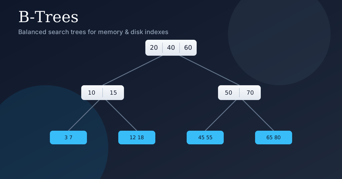
B-trees solve that problem by getting wide. Each node holds many sorted keys and can point to many children. A lookup does more work inside the page it already has and needs far fewer page reads on the way down.
That shape is why B-tree variants show up in PostgreSQL, MySQL, SQLite, filesystems, and embedded stores. Most databases actually use a B+tree, with records in the leaves and separator keys above them. I’m using the classic B-tree here because the balancing operations are easier to see.
Five rules keep the tree balanced
Choose a minimum degree t of at least 2. Then:
- Every node has at most 2t − 1 keys.
- Every node except the root has at least t − 1 keys.
- The root has at least one key unless the tree is empty.
- A non-leaf with k keys has exactly k + 1 children.
- All leaves sit at the same depth.
- Keys inside a node are sorted; subtree i holds keys between key i−1 and key i.
When t is 2, each non-root node holds between one and three keys. This is also called a 2-3-4 tree.
Break one yourself
Insert, search, and delete a few values below. The animation marks the path before it changes the tree. Try a different value of t and watch the same keys settle into a wider or narrower shape.
Run an operation above and every step lands here — scrub, replay, or slow it down.
Try insert, search, or delete — each walk animates the path so nodes don't just pop in.
The three operations
The pseudocode uses CLRS-style notation: t is the minimum degree, x.n is the number of keys, x.key[1..n] contains those keys in order, x.c[1..n+1] contains child pointers, and x.leaf says whether the node is a leaf.
Search
B-TREE-SEARCH(x, k)
  i ← 1
  while i ≤ x.n and k > x.key[i]
    i ← i + 1
  if i ≤ x.n and k = x.key[i]
    return (x, i)                 // found
  if x.leaf
    return NIL                    // not found
  else
    DISK-READ(x.c[i])             // or memory fetch
    return B-TREE-SEARCH(x.c[i], k)
One node can rule out a large range of keys before the next fetch. That is the whole win.
Insert
An insert ends in a leaf. The useful trick is to split a full child before descending into it. That way the recursive call never has to deal with a full node.
B-TREE-SPLIT-CHILD(x, i)
  // x.c[i] is full (2t − 1 keys). Split it around the median.
  y ← x.c[i]
  z ← ALLOCATE-NODE()
  z.leaf ← y.leaf
  z.n ← t − 1
  for j ← 1 to t − 1
    z.key[j] ← y.key[j + t]
  if not y.leaf
    for j ← 1 to t
      z.c[j] ← y.c[j + t]
  y.n ← t − 1
  // shift x's children/keys right and promote median y.key[t]
  insert z as x.c[i + 1]
  insert y.key[t] as x.key[i]
  y loses key[t] and the moved children
  DISK-WRITE(y); DISK-WRITE(z); DISK-WRITE(x)

B-TREE-INSERT(T, k)
  r ← T.root
  if r.n = 2t − 1
    s ← ALLOCATE-NODE()
    T.root ← s
    s.leaf ← FALSE
    s.n ← 0
    s.c[1] ← r
    B-TREE-SPLIT-CHILD(s, 1)
    B-TREE-INSERT-NONFULL(s, k)
  else
    B-TREE-INSERT-NONFULL(r, k)

B-TREE-INSERT-NONFULL(x, k)
  i ← x.n
  if x.leaf
    shift keys right to open slot for k
    x.key[i + 1] ← k
    x.n ← x.n + 1
    DISK-WRITE(x)
  else
    while i ≥ 1 and k < x.key[i]
      i ← i − 1
    i ← i + 1
    DISK-READ(x.c[i])
    if x.c[i].n = 2t − 1
      B-TREE-SPLIT-CHILD(x, i)
      if k > x.key[i]
        i ← i + 1
    B-TREE-INSERT-NONFULL(x.c[i], k)
The median moves up to the parent, and the keys on either side become two children. If the root is full, it splits too and the tree grows by one level.
Delete
Deletion is the fiddly one. Before descending into a child that has only t − 1 keys, give it room to lose a key: borrow from a sibling if possible, otherwise merge it with a sibling.
B-TREE-DELETE(x, k)
  find index i where k would live in x

  if k is in x:                                   // case: key in this node
    if x.leaf
      remove k from x
    else if x.c[i] has ≥ t keys
      k' ← predecessor(k) in x.c[i]
      x.key[i] ← k'
      B-TREE-DELETE(x.c[i], k')
    else if x.c[i + 1] has ≥ t keys
      k' ← successor(k) in x.c[i + 1]
      x.key[i] ← k'
      B-TREE-DELETE(x.c[i + 1], k')
    else
      merge x.c[i], k, and x.c[i + 1]
      B-TREE-DELETE(x.c[i], k)
  else if x.leaf
    return                                        // missing key
  else
    // ensure child we descend into has ≥ t keys
    if x.c[i] has only t − 1 keys
      borrow from a sibling or merge with one
    B-TREE-DELETE(appropriate child, k)

  if root has 0 keys and is not a leaf
    T.root ← its only child                       // tree shrinks by one level
Borrowing rotates a parent separator down and a sibling key up. Merging pulls the separator between two small children and turns all three pieces into one node. If that empties the root, its only child becomes the new root and the tree loses a level.
What this has to do with a database index
Imagine a users table spread across unsorted heap pages. Without an index, WHERE id = 36 starts at page one and keeps reading until it finds the row. A miss scans everything.
A secondary index—usually a B+tree—keeps the IDs ordered. Its leaf entry points to the heap page or row that contains the full record. Now the database can:
- Walk a handful of index nodes from the root (one I/O each, unless cached).
- Read the referenced heap page for the row, unless the index already covers the query.
On a large table, that is the difference between a linear pile of page reads and a handful of index reads plus one trip to the heap.
Watch the page reads
This demo puts 24 rows into heap pages of four rows each and builds an index on id. Run a table scan, then use the index for the same value. The existing IDs are multiples of three from 3 through 72. Searching for 69 makes the scan do nearly all the work; 33 ends sooner, while 11 shows the cost of a miss.
Heap table (users)
Rows sit in insertion order across 6 pages (4 rows/page). A scan walks pages one-by-one until it hits the id — each new page is another I/O.
| Page | id | name | city |
|---|---|---|---|
| 1 | 3 | Ava | Austin |
| 1 | 6 | Ben | Berlin |
| 1 | 9 | Cora | Chicago |
| 1 | 12 | Drew | Dublin |
| 2 | 15 | Elena | Edmonton |
| 2 | 18 | Finn | Florence |
| 2 | 21 | Gina | Austin |
| 2 | 24 | Hugo | Berlin |
| 3 | 27 | Iris | Chicago |
| 3 | 30 | Jules | Dublin |
| 3 | 33 | Kara | Edmonton |
| 3 | 36 | Leo | Florence |
| 4 | 39 | Mia | Austin |
| 4 | 42 | Noah | Berlin |
| 4 | 45 | Omar | Chicago |
| 4 | 48 | Pia | Dublin |
| 5 | 51 | Quinn | Edmonton |
| 5 | 54 | Rosa | Florence |
| 5 | 57 | Sam | Austin |
| 5 | 60 | Tess | Berlin |
| 6 | 63 | Uma | Chicago |
| 6 | 66 | Vince | Dublin |
| 6 | 69 | Willa | Edmonton |
| 6 | 72 | Xander | Florence |
Secondary memory index on id
The B-tree stores keys (and, in a real engine, pointers to heap pages). Height stays small, so lookups cost a few node reads.
Default 69 sits late in the heap (scan reads many pages). Try 33 for a shorter scan, or 11 for a miss. Run both modes on the same id.
Run an operation above and every step lands here — scrub, replay, or slow it down.
Simulated page I/O
0/ 6 heap pages
Pick a lookup id, then run Table scan or Use B-tree index to watch each page read.
Real engines add plenty that this toy leaves out:
- B+trees keep all row pointers in leaves and link leaves for range scans (
BETWEEN,ORDER BY). - Internal nodes store separator keys sized to fill a page (often 4–16 KiB).
- Buffer pools cache hot root/upper levels so common lookups barely touch disk.
- Concurrent access uses latch coupling / leaf locks; splits and merges become careful atomic operations.
- Covering indexes can answer queries from the index alone — no heap fetch.
But the useful mental picture stays the same: a wide, balanced index replaces a linear hunt with a short walk.
Costs at a glance
| Operation | I/O / node visits | Notes |
|---|---|---|
| Search | O(logₜ n) | One node per level |
| Insert | O(logₜ n) | O(1) page operations per level for fixed-size pages; O(t) in-node copying |
| Delete | O(logₜ n) | Borrow/merge along the path |
| Range scan (B+tree) | O(logₜ n + k) | k leaf entries after the first |
Space is O(n). The constants hide page size, key width, and caching, which is why a B-tree can be the better real-world choice even though a hash index offers O(1) average point lookups.
When I’d choose one
B-trees are a natural fit when keys need to stay ordered for ranges, scans, or ORDER BY, and when nodes line up with pages or blocks. They stay balanced while keys come and go, without periodically rehashing the entire structure.
For equality-only lookups, a hash index may be simpler and faster. For sustained write-heavy workloads, an LSM tree may be worth its read and compaction costs. For a read-heavy relational index that also needs ranges, B+trees remain the unsurprising default.
If you want the idea to stick, grow the first tree until it splits, then delete until two nodes merge. After that, compare the scan and index I/O counts. “Index Scan” in an EXPLAIN plan feels much less abstract once you can picture the pages it avoids.